Prelab
In order to implement and test the PID controller through my labtop, I set up a few bluetooth commands for communication between the robot and the computer. SET_VALS allows the user to change the PID controller values on the jupyter notebook directly, rather than uploading the .ino code to Artemis everytime one value is changed.
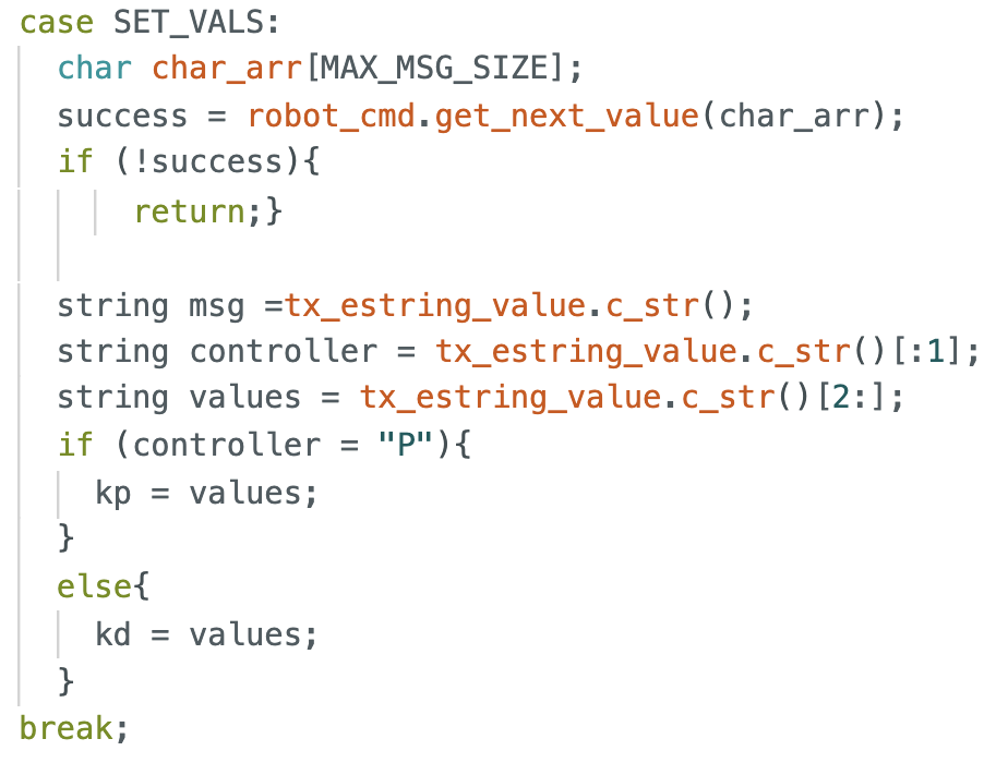
The user has to define which controller it is changing and the value corresponding to the controller. (i.e. "P:0.05"). For the PID control task, PID_CONTROL starts the task: robot going towards the wall and stopping at a certin setpoint (300mm).
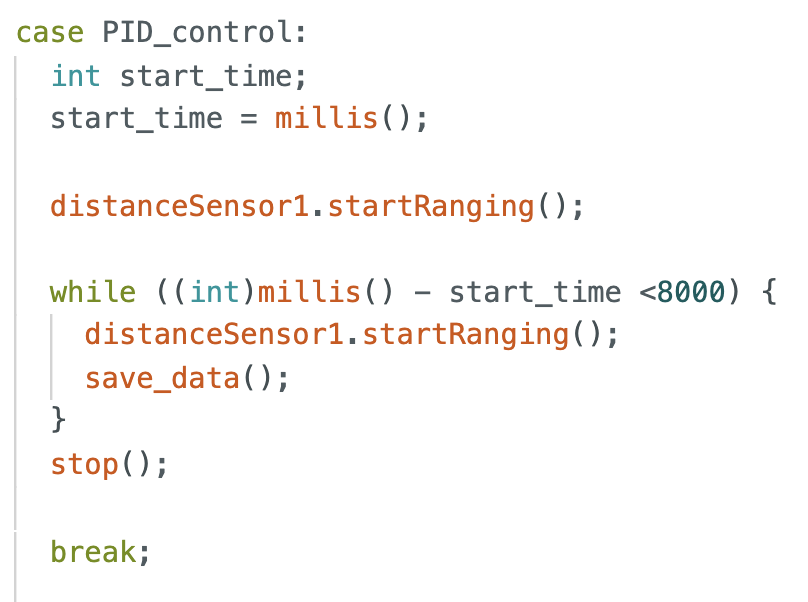
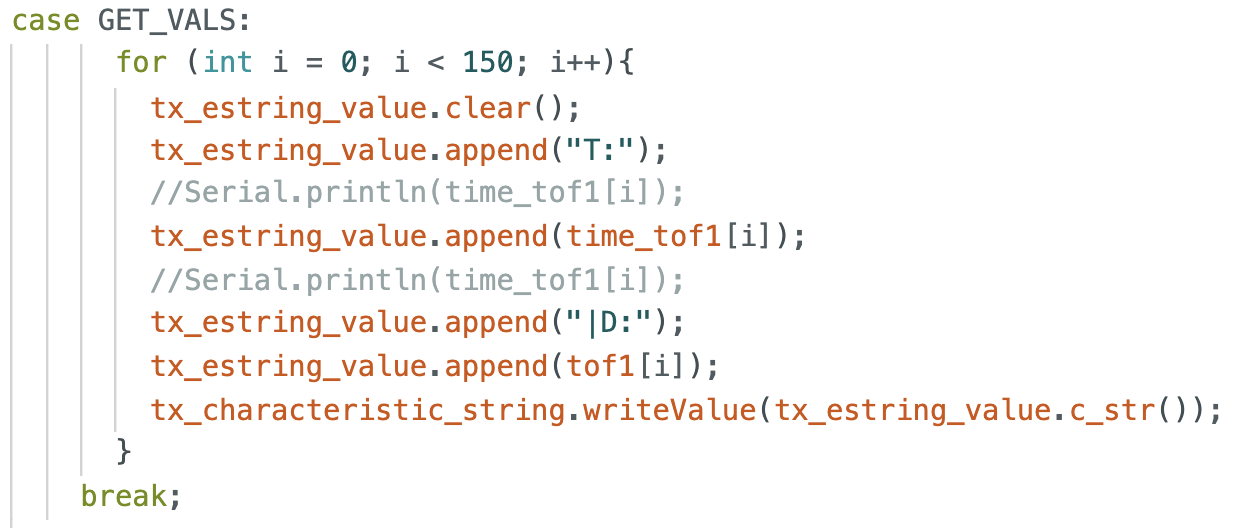
After the task as been performed, GET_VALS command allows the user to retrieve the stored data in the Artemis of the stunt. Using the notification handler, the values are stored in corresponding arrays in python and later graphed.
Task A: Position Control
For data collection during the robot performance. I stored the individual data points in the Artemis while the tasking is performed, and the aggregate data was sent to the computer via bluetooth after the task has ended. I used arrays of size 150 (it was never all used up) to store time, motor PWM input and distance sensor values. Initially, I only used the P controller, but found that it always stopped about 30 mm away from the setpoint. Thus, I finalized with PD controller. During the task, the function pid() calculates the new speed,
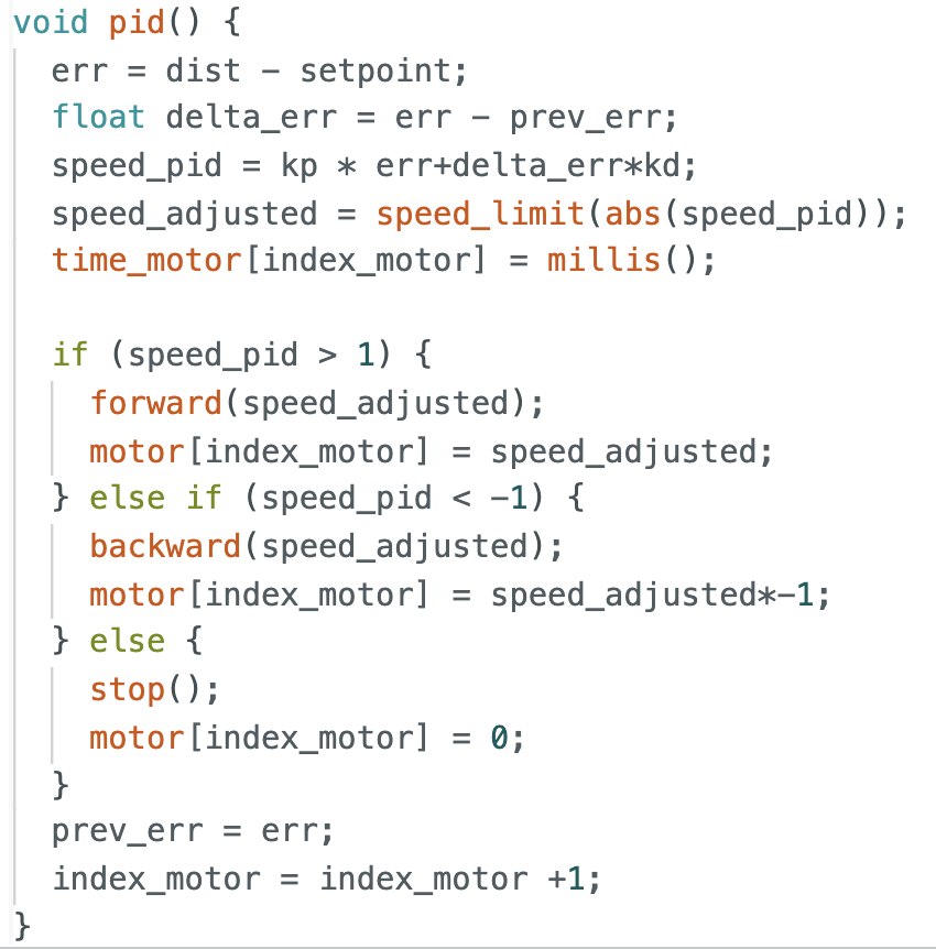
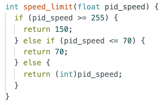
and uses the function speed_limit() to ensure that the roobt still moves even if it is bigger than the maximum or smaller than the minimum.
How to find appropriate Kp value
First, the Kp values were found by approximate calculating what the pid_speed would be throughout the run if the robot starts approximately at 1600mm. Since the set point was 300mm, the error at the beginning will be 1300. To achieve a maximum PWM of 250, the ideal starting Kp value should be 250/1300 = 0.192.
P Control
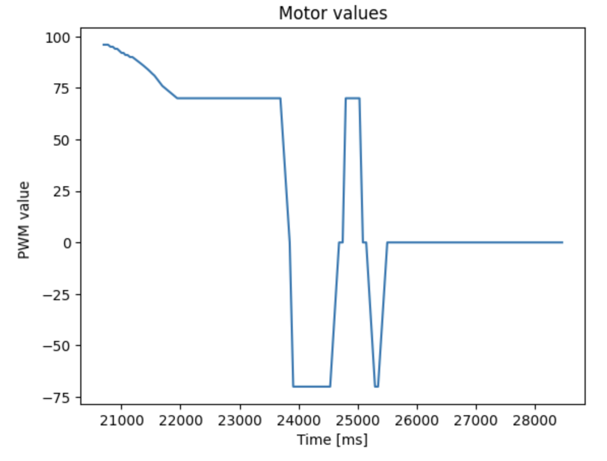
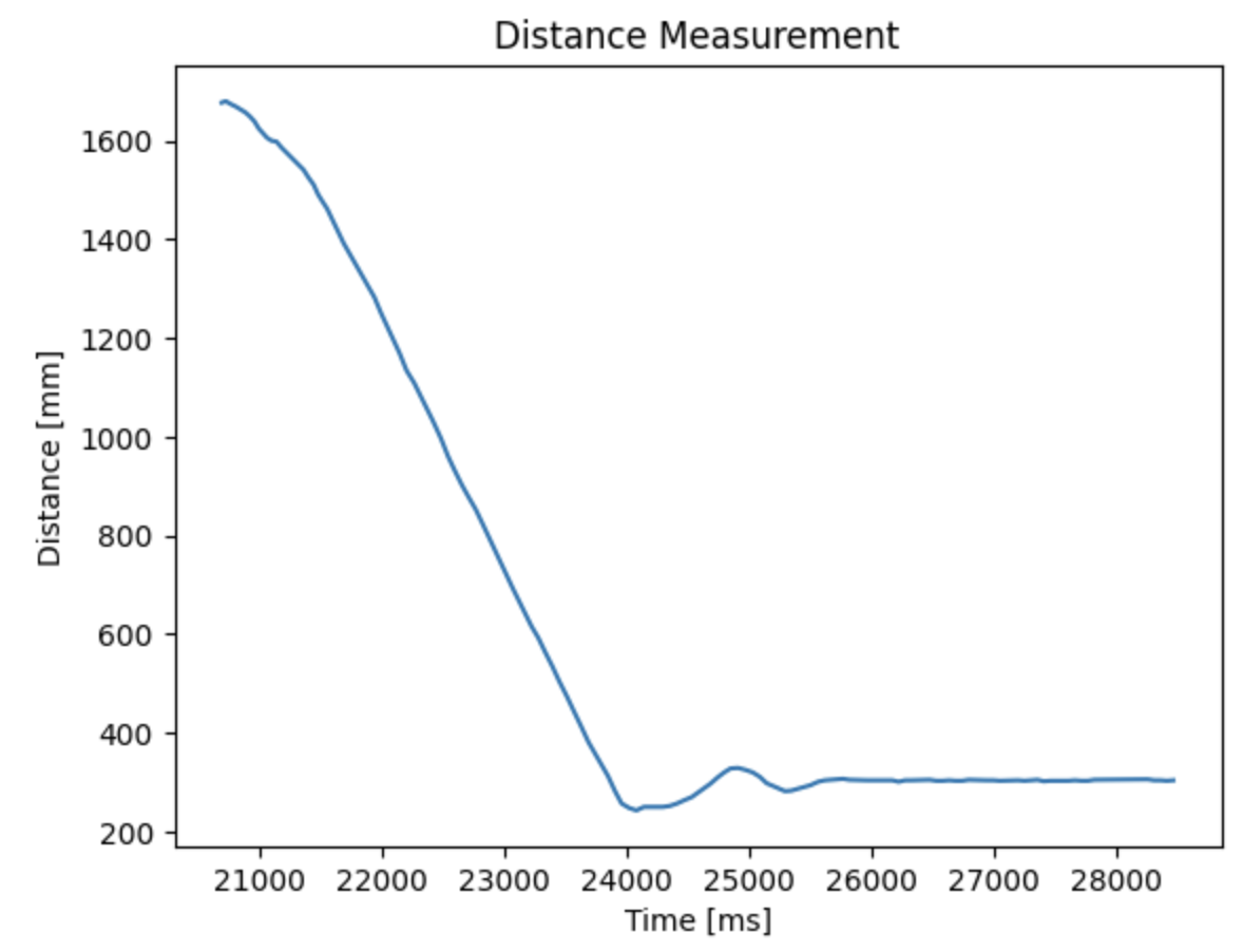
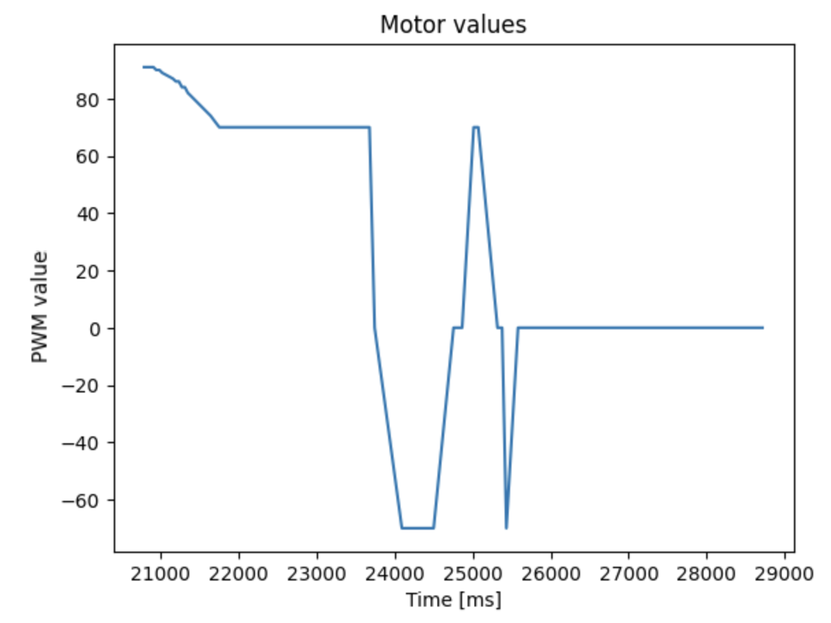
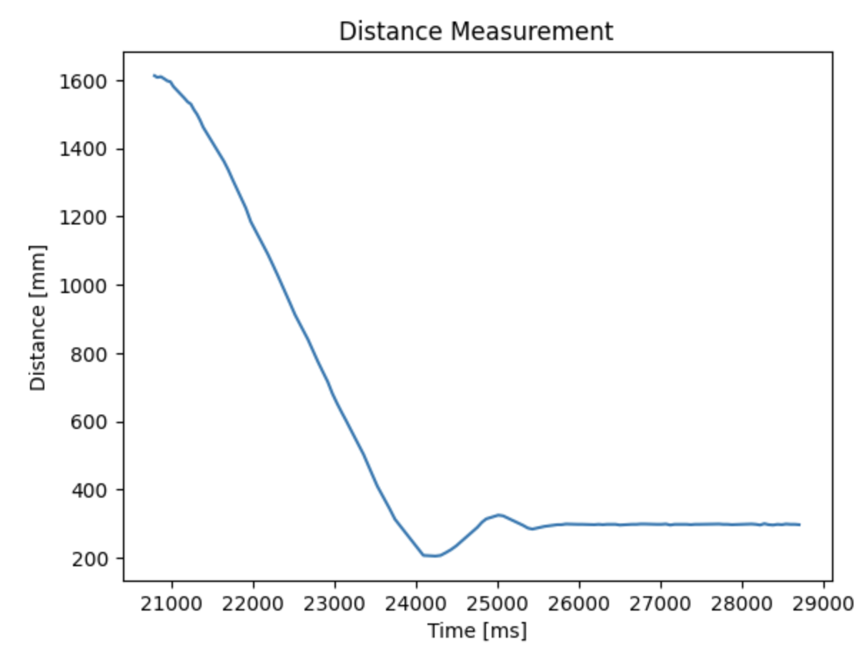
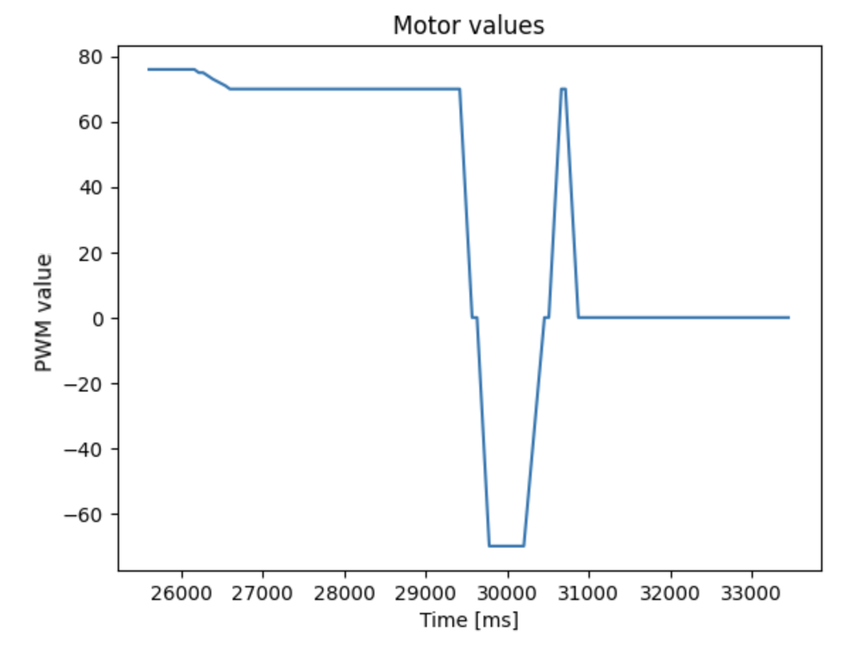
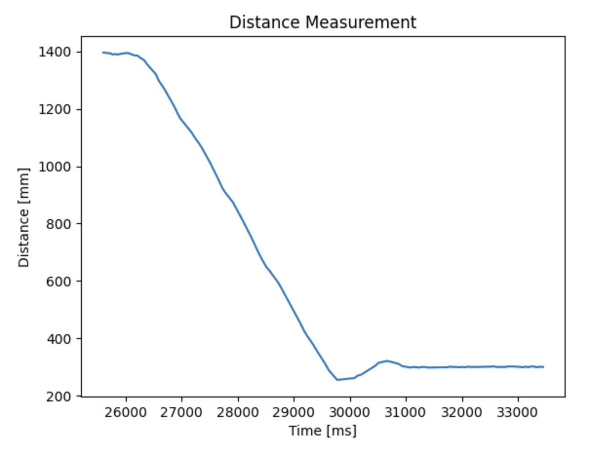
I first started with a P control, since it is the most simple controller choice. After a lot of trial and error, I finalized with a Kp value of 0.09. If the Kp value was bigger, the velocity of the car was higher, but the car was very close to crashing due to a large overshoot. For example, a Kp value above 0.18 made the car crash to the wall.
Starting at Kp value of 0.19, I slowly decreased the Kp value that will allow me to have stable results. The reason why values near 0.19 was too unstable is due to the long update time for the ToF sensors (based on the data collected, I gathered ~100 tof points during one trial that took about 8 seconds -- meaning the update time was around 80 ms.) Below are the videos and the resulting graphs from the test.
PD Control
To additionally implement a derivative control, I calculated the derivative and implemented it in the PID_control. I chose the derivative control since it is relatively easy to implement and I don't have to worry about the integrator wind-up in integral control.
How to find appropriate Kd value
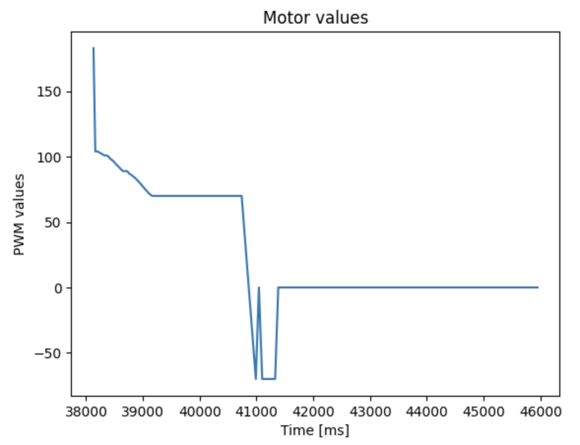
The main reason I added derivative control was to eliminate the steady state error that occurred during my P control. Rather than estimating an ideal Kd value, I slowly increased the Kd value from 0 to eliminate the steady state error and decrease the large overshoot seen in P control.
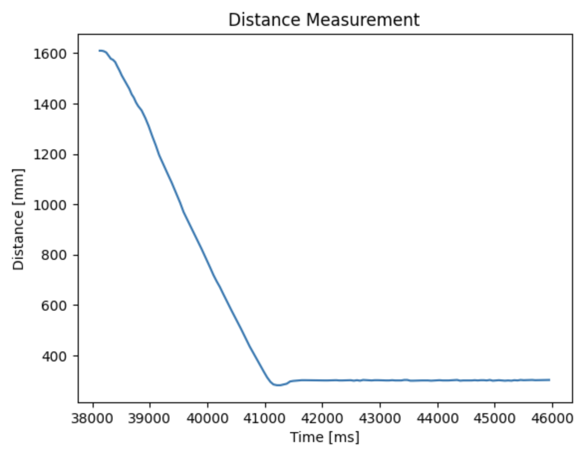
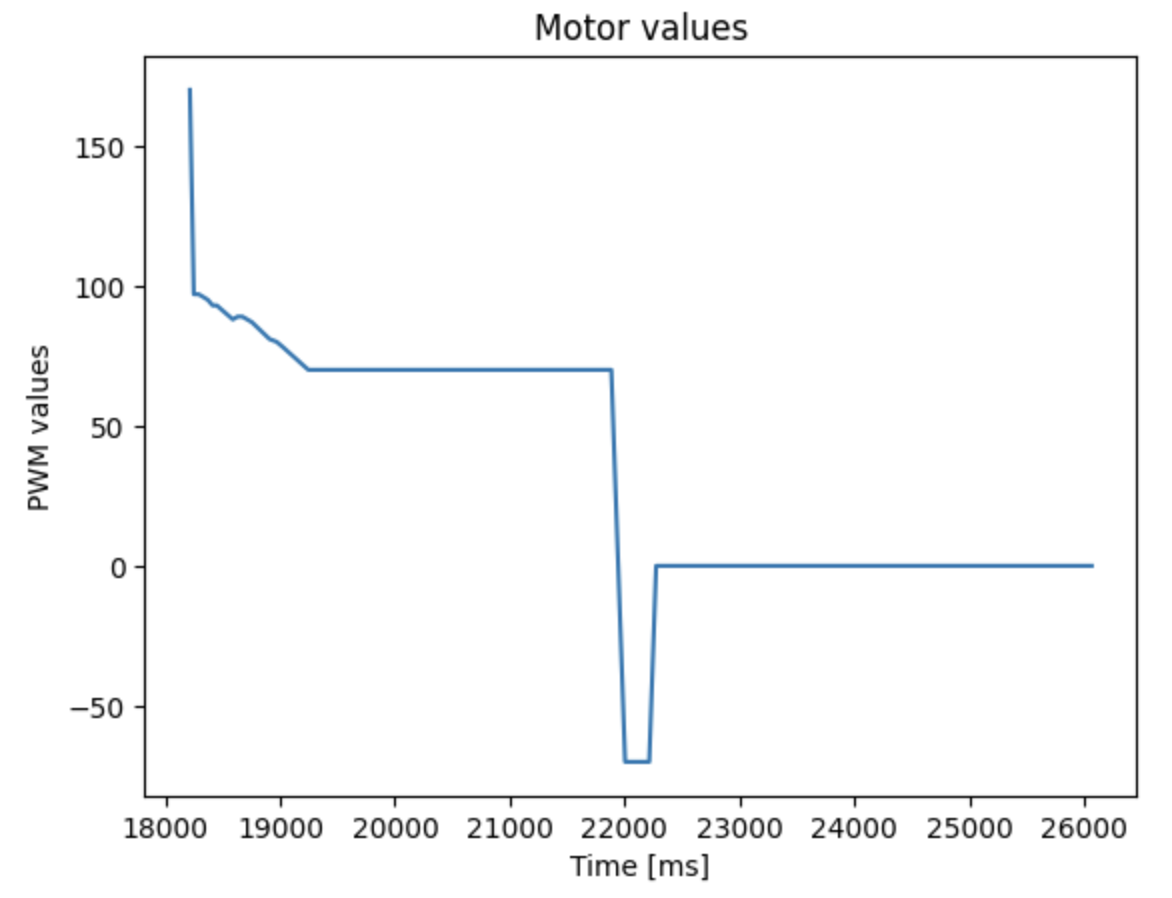
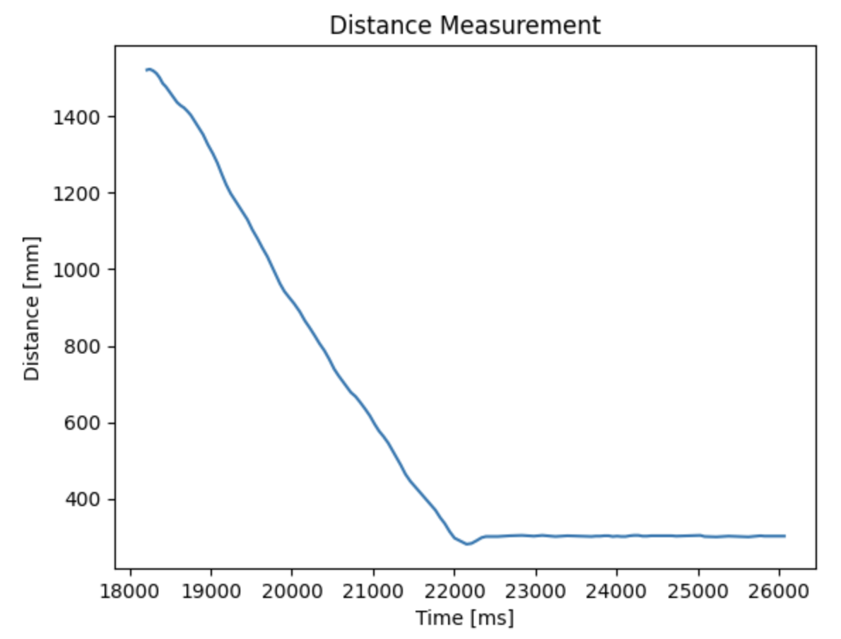
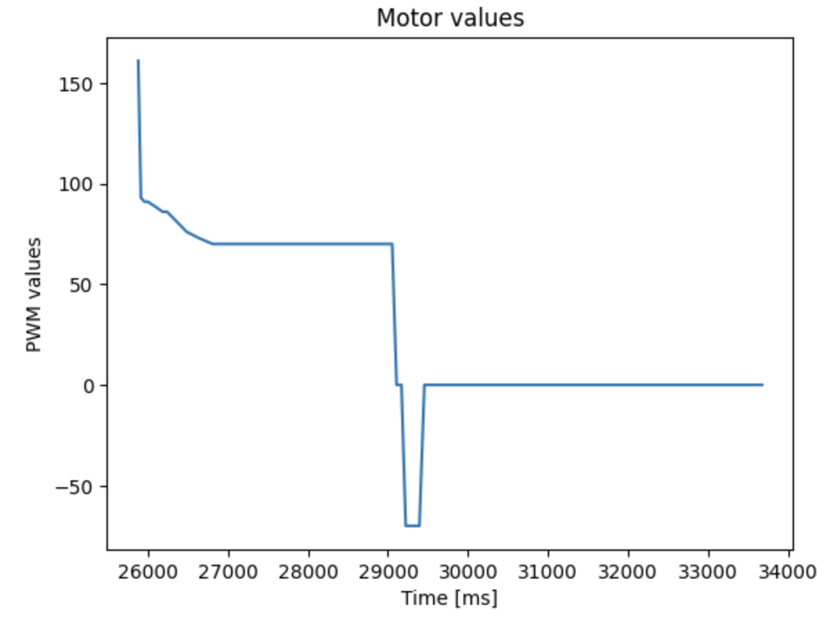
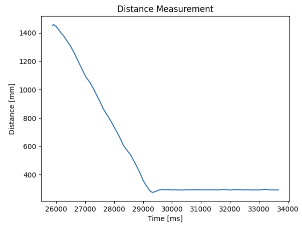
The finalized Kp and Kd values were Kp = 0.09, Kd = 0.06. Below are the graphs and the implementation video.
Conclusion
For each controller test, all three trials gave similar results. For P controller, there was a larger overshoot, and therefore longer time to stop at the setpoint. In the video, it can be seen through the the back-and-forth motion that the robot makes around the 300 mm point. Comparatively, the PD controller had a smaller overshoot and found its position relatively quickly than the P controller. The P controller took around 5.5 seconds to stabilize and the PD controller took around 4.5 seconds to stabilize.
Ultimately, the maximum speed acheived was 0.7 m/s, with an average of 0.3 m/s throughout the run. The major setback to more efficient pid control was the very slow sampling rate of ~80 ms for 1 sensor reading that limited the efficiency of control.
I only sent the collected data once after the task was complete since the task was short (maximum 8 seconds - including steady state) and there were only 4 arrays of 150 data points to send at the end, although I never used the full capacity. However, if I have a longer task later on, I would have to send the data during the task if I need to.