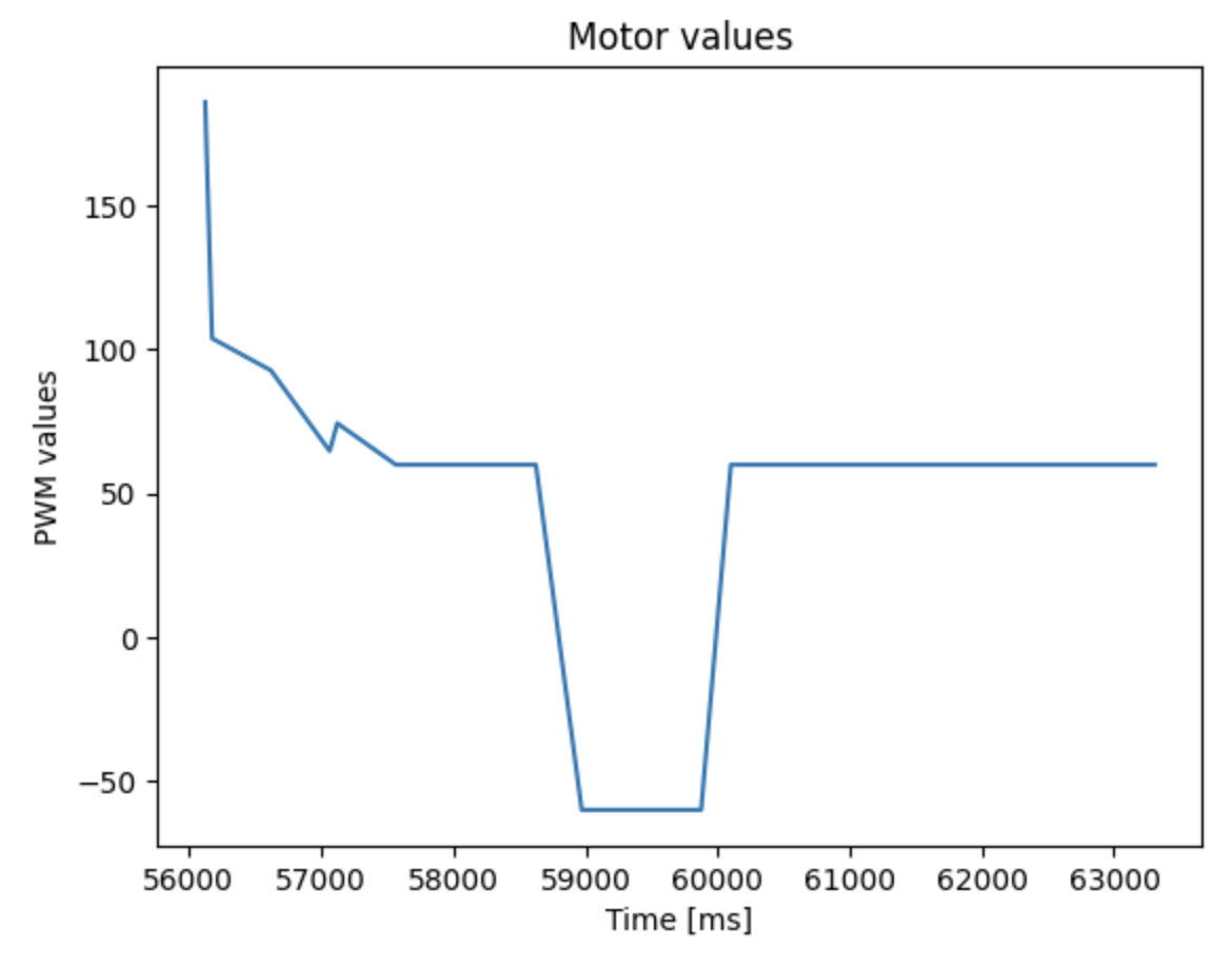
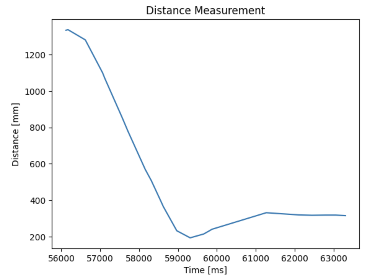
Estimating drag and momentum
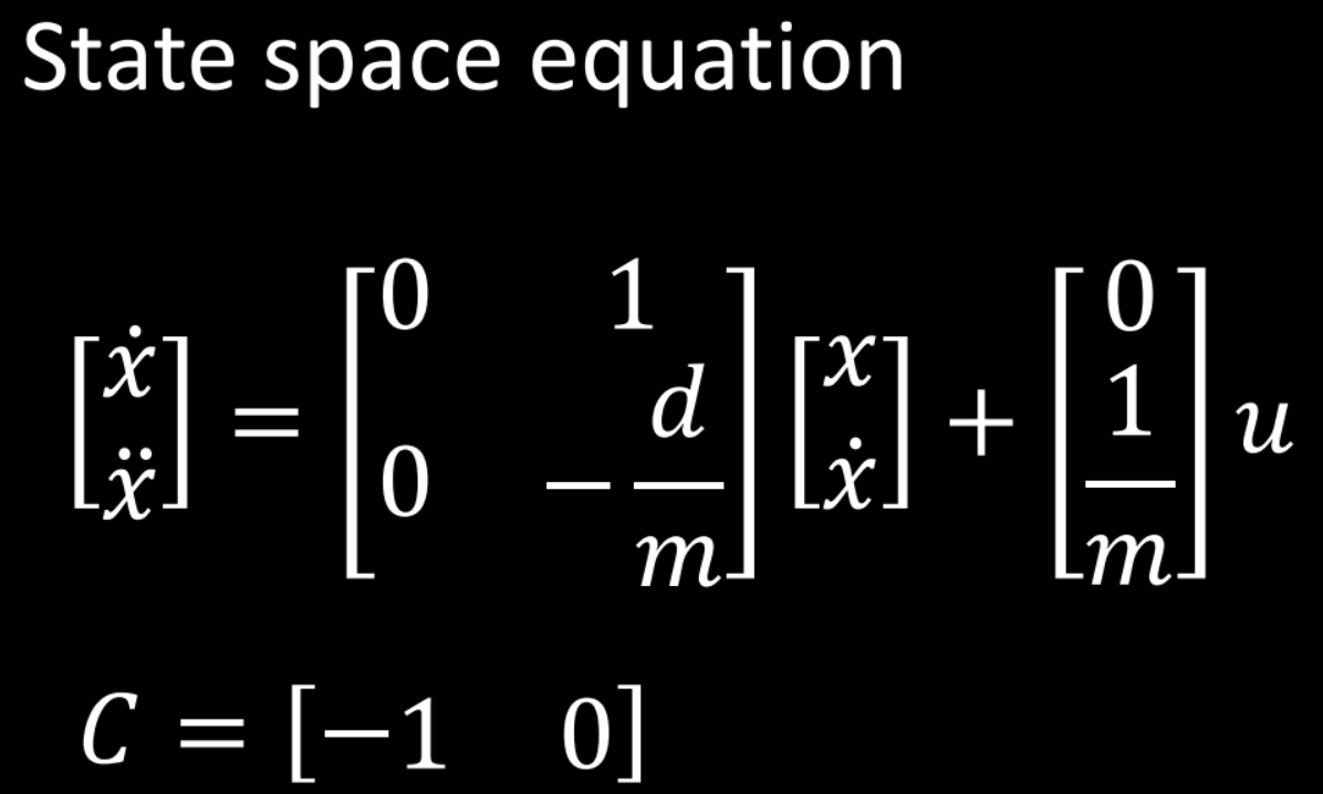
In order to build the state space model for my system, I had to estimate the drage and momentum terms for the A and B matrices (as written below). This was done by driving the car towards a wall while logging my motor and ToF sensor output.
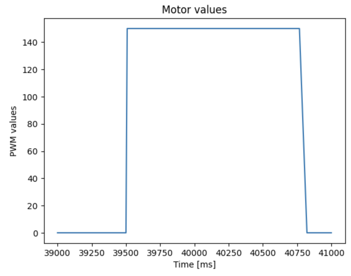
I decided on my step size using the maximum PWM value that was produced during my lab 6, which was around 150. Thus, I gave the 150 PWM input to the motor until the car reached 100cm away from the wall. (PWM input shown below)
Below are the ToF sensor output and the computed speed of the car during the step input.
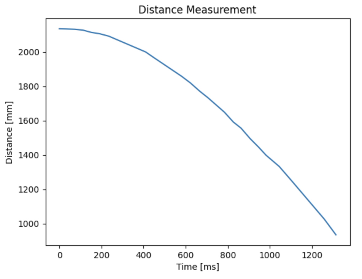
The maximum speed reached was 1654 mm/s with PWM value of 150. Using the data, the steady state speed and the 90% rise time was found to be around 1654 mm/s and 1.27 s, respectively.
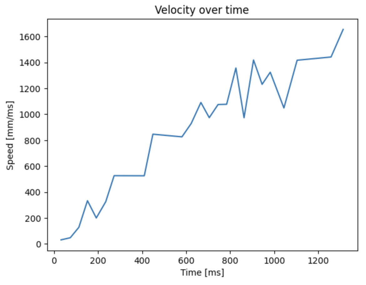
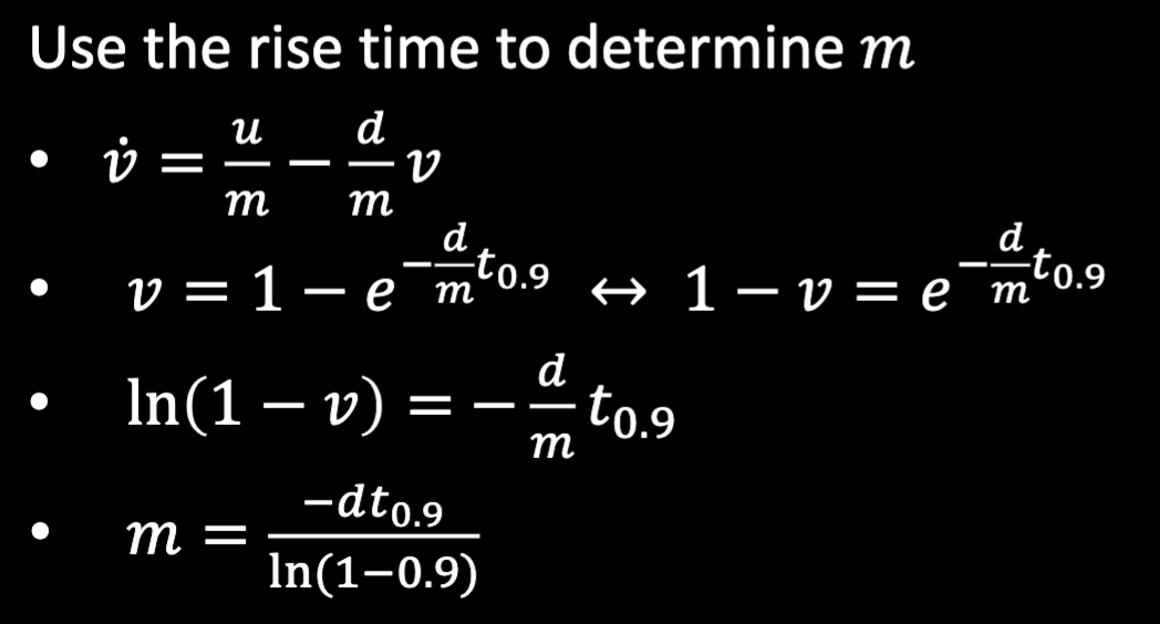
Using the data obtained above, I implemented the Kalman Filter in Jupyter, by finalizing my A and B matrices using the steady state velocity and 90% rise time. To figure out d term (drag) of the system, we can calculate it using the steady state velocity (1654 mm/s) and u as 1. Thus, the d term came out to be ~0.00060.

Using the 90% rise time and the d term, the m term came out to be 0.00033.
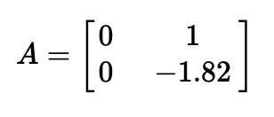
Initializing KF
With the newly found d and m values, I plugged them into the matrices to finalize the KF setup.
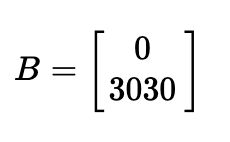
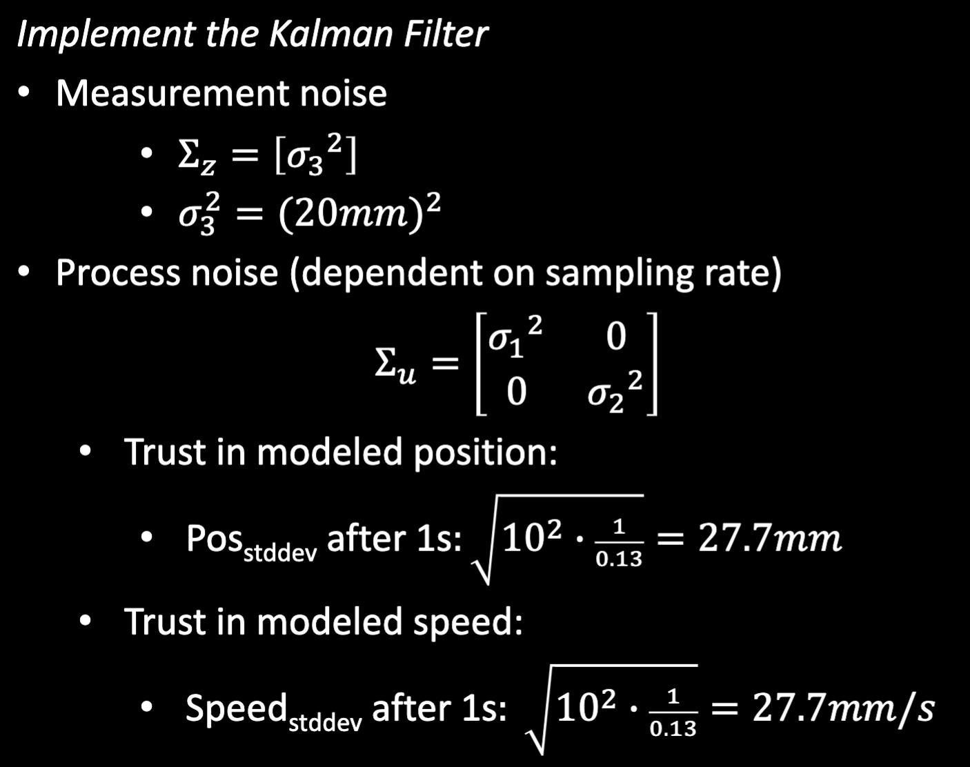
Since the KF needs process and measurement noise covariance matrices, I used the following equations to approximate the noise covariance values using the sampling rate. Since my sampling rate is ~0.18s, I substituted that value to finalize all matrices needed for the KF implementation.


Implementing KF in Jupyter
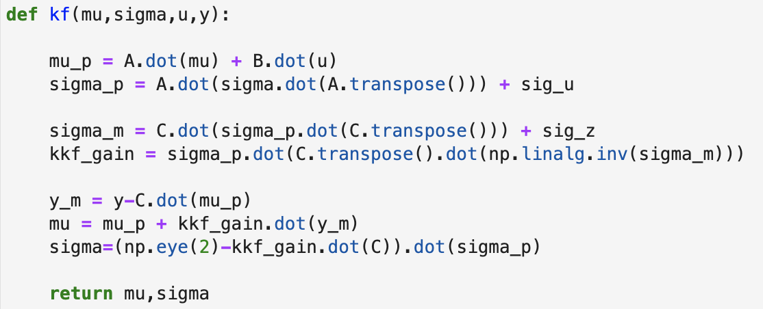
Now that the Kalman filter is ready, I iterated over the ToF values that I already had from lab 6 and applied the KF code. Through using the following functions and codes, I was able to implement the kalman filter onto the data that I collected during the PID control lab. I first initialized all the matrices (A, B, C and the noise covariance matrices),
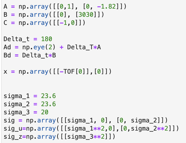
and used the kf function to get the filtered data.
This is the result of the Kalman filter. The blue line is the raw data taken from the sensor on the car, and the orange line is the data produced by the KF. I used the kalman filter using different sigma values for different level of uncertainty of the model and the sensors.
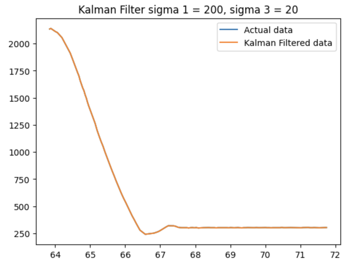
This is when I gave more trust to the sensor output. Thus, it believed in the sensor output values, which is why the kalman filter data and the raw data are very similar to each other.
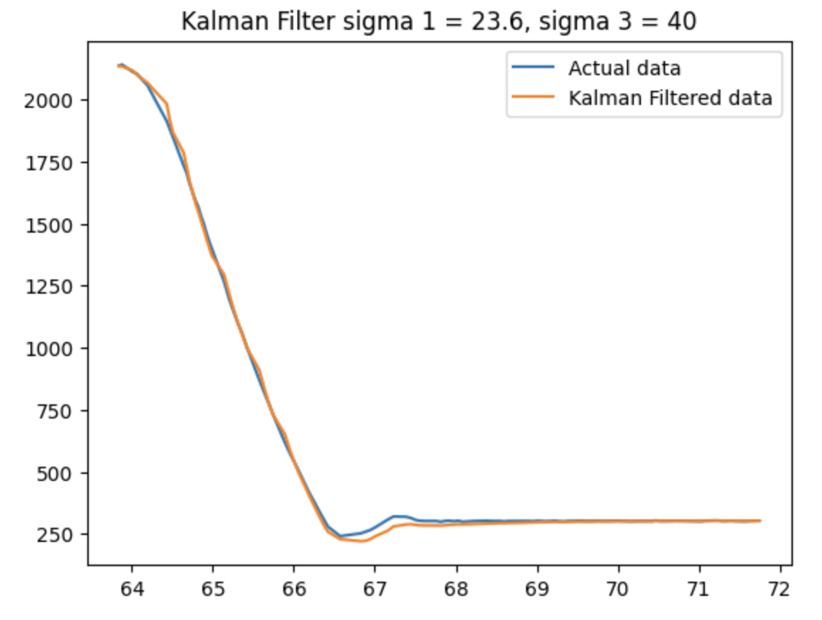
When higher trust/certainty is given to the model, the filtered values deviate from the raw data, especially during the overshoot portion of the graph. It slightly increased the overshoot time and magnitude and slowly converged to the constant equilibrium distance.
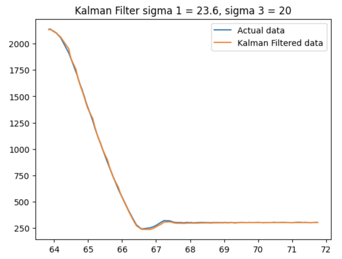
I ended up using the standard values that the lecture recommended using the sensor ranging time, because I didn't trust the sensor too much due to its frequency inaccuracies, but the model could also be faulty sometimes. Thus, by using the default values of uncertainties, I can later experience the balance of accuracy between the sensor and the model and decide later on by tweaking the individual sigma values.
Extrapolation
I chose to implement the extrapolation method to my sensor data since the kf filter implementation was not stable enought. The linear extrapolation can speed up the controller since the robot does not have to wait for the next ToF sensor to change the motor PWM values; rather, it can estimate its current position using linear extrapolation and use the controller even when the ToF sensor is not updated.
Using the code snippets attached below, I got the robot to conduct the pid controller, using the extrapolation method this time.

Using this method, the robot can estimate the current position from the wall in between the time the ToF sensor updates, which takes a significant amount of time considering the robot's fast speed. Thus, the extrapolate method is called during the time ToF sensor is updating, and using that value the pid controller decides on the next PWM motor value to change.
Below are the videos and the distance vs time graph from the pid controller with the extrapolation method this time.
